import numpy as np
import matplotlib.pyplot as plt
from matplotlib.colors import LogNorm, LinearSegmentedColormap, Normalize, SymLogNorm
from matplotlib import cm as colormap
import time
from string import ascii_lowercase

# SimPEG, discretize/
import discretize
from discretize import utils
from SimPEG.electromagnetics import time_domain as tdem
from SimPEG.electromagnetics import resistivity as dc
from SimPEG.utils import mkvc, plot_1d_layer_model
from SimPEG import (
    maps,
    data,
    data_misfit,
    inverse_problem,
    regularization,
    optimization,
    directives,
    inversion,
    utils,
)

from pymatsolver import Pardiso
csx = 10
csz = 5
pf = 1.3
ncx = 15
ncz = int(500/csz)
ncza = 12
npadx = 21
npadz = 23
mesh = discretize.CylindricalMesh(
[[(csx, ncx), (csx, npadx, pf)], [np.pi*2], [(csz, npadz, -pf), (csz, ncz+ncza), (csz, npadz, pf)]],
origin = "000"
)
mesh.origin = np.r_[0, 0, -mesh.h[2][:npadz+ncz].sum()]
mesh.plot_grid()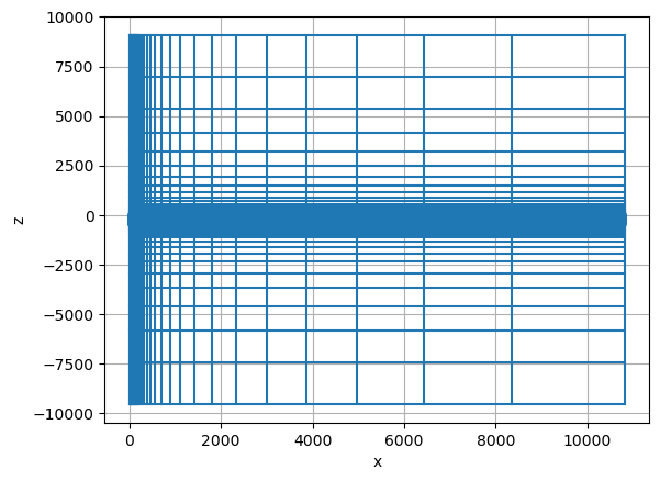
rho_back = 100
sigma_target = np.r_[1./rho_back, 0.1, 1, 10, 100]
target_radius = np.r_[0, np.inf]
target_t = 30
target_z = -150+ target_t/2 * np.r_[-1, 1]
sigma_air = 1e-8

tx_height = 30
tx_radius = 10

def diffusion_distance(sigma, t):
    return 1260 * np.sqrt(t/sigma)
rx_times = np.logspace(np.log10(2e-5), np.log10(8e-3), 20)
diffusion_distance(1./rho_back, rx_times[-1])1126.9782606598942models = {}
for sig in sigma_target:
key = f"sigma_{sig:1.0e}"
m = sigma_air * np.ones(mesh.n_cells)
m[mesh.cell_centers[:, 2] < 0] = 1./rho_back
inds_target = (
(mesh.cell_centers[:, 0] < target_radius.max()) &
(mesh.cell_centers[:, 0] > target_radius.min()) &
(mesh.cell_centers[:, 2] < target_z.max()) &
(mesh.cell_centers[:, 2] > target_z.min())
)
m[inds_target] = sig
models[key] = mfig, ax = plt.subplots(1, len(models), figsize=(3*len(models), 2))
xlim = 500*np.r_[-1, 1]
zlim = np.r_[-800, 100]
for i, key in enumerate(models.keys()):
plt.colorbar(mesh.plot_image(
models[key], ax=ax[i],
pcolor_opts={"norm":LogNorm(vmin=sigma_air, vmax=sigma_target.max())},
mirror=True
)[0], ax=ax[i])
ax[i].set_xlim(xlim)
ax[i].set_ylim(zlim)
plt.tight_layout()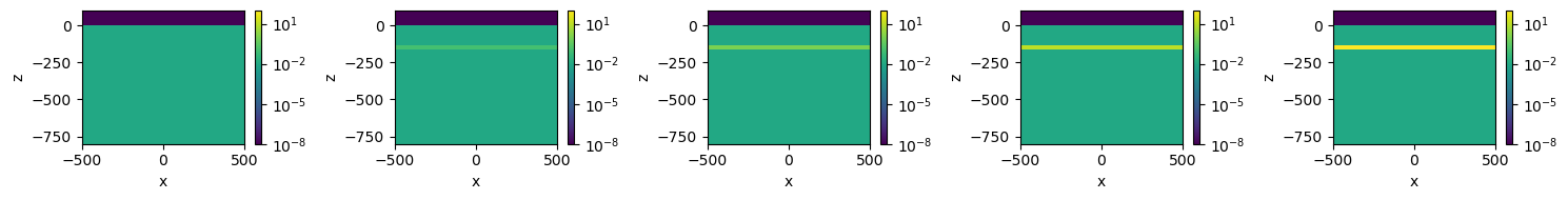
fig, ax = plt.subplots(1, 1, figsize=(4.5, 3.5))

xlim = 500*np.r_[-1, 1]
zlim = np.r_[-450, 100]

key = "sigma_1e+00"
cb = plt.colorbar(mesh.plot_image(
    models[key], ax=ax,
    pcolor_opts={"norm":LogNorm(vmin=sigma_air, vmax=1e2), "cmap":"Spectral_r"},
    mirror=True
)[0], ax=ax)
ax.set_xlim(xlim)
ax.set_ylim(zlim)
cb.set_label("conductivity (S/m)")

plt.tight_layout()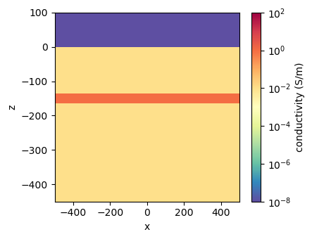
simulation
waveform=tdem.sources.StepOffWaveform()
# waveform=tdem.sources.VTEMWaveform()

rx_z = tdem.receivers.PointMagneticFluxTimeDerivative(
    np.r_[0, 0, tx_height], times=rx_times, orientation="z"
)

src = tdem.sources.CircularLoop(
    location=np.r_[0, 0, tx_height], radius=tx_radius, receiver_list=[rx_z], waveform=waveform
)

survey = tdem.Survey([src])
# waveform.peak_time/1e-4time_steps = [
# (1e-4, np.floor(waveform.peak_time/1e-4)),
# (1e-5, np.floor((waveform.off_time-waveform.peak_time)/1e-5)),
(1e-5, 40), (3e-5, 20), (1e-4, 20), (3e-4, 20)
]sim = tdem.simulation.Simulation3DElectricField(
mesh=mesh, survey=survey, time_steps=time_steps, solver=Pardiso,
sigmaMap=maps.IdentityMap(mesh)
)fig, ax = plt.subplots(1,1)
ax.plot(sim.times*1e3, [waveform.eval(t) for t in sim.times])
ax.plot((rx_times+waveform.off_time)*1e3, np.zeros_like(rx_times), "|k")
ax.plot(sim.times*1e3, -0.1*np.ones_like(sim.times), "|r")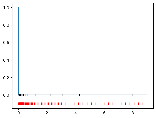
fields = {}
dpred = {}

for key, val in models.items():
    t = time.time()
    fields[key] = sim.fields(val)
    dpred[key] = sim.dpred(val, f=fields[key])
    print(f"done {key}... {time.time() - t: 1.2e}s")
done sigma_1e-02...  3.50e+00s
done sigma_1e-01...  8.59e-01s
done sigma_1e+00...  1.13e+00s
done sigma_1e+01...  1.01e+00s
done sigma_1e+02...  9.95e-01s
fig, ax = plt.subplots(1, 1, figsize=(4.5, 3.5))
highlight = None
for i, key in enumerate(list(dpred.keys())[:3]):
    val = dpred[key]
    if i == 0:
        color = "--k"
        label="background"
    else:
        color = f"C{i-1}"
        label = f"{float(key.split('_')[-1]):1.1f} S/m"
    ax.loglog(rx_times*1e3, -val, color, label=label, alpha=1 if highlight == i or highlight is None else 0.2)

ax.set_xlim(5e-2, 10)
# ax.set_ylim(1e-14, 4e-10)
ax.legend()
ax.set_xlabel("time (ms)")
ax.set_ylabel("db/dt")
ax.grid(alpha=0.7)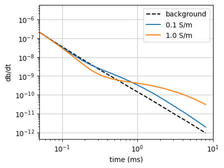
dpred1d = {}

for i, sig in enumerate(sigma_target):
    key = f"sigma_{sig:1.0e}"
    dpred1d[key] = sim1d_true.dpred(np.log(np.r_[1./rho_back, sig, 1./rho_back]))
m_true = np.log(np.r_[1./rho_back, 0.1, 1./rho_back])
sim1d_true = tdem.Simulation1DLayered(
survey=tdem.Survey([src]), thicknesses=np.r_[-target_z.max(), np.diff(target_z)], sigmaMap=maps.ExpMap(nP=3)
)
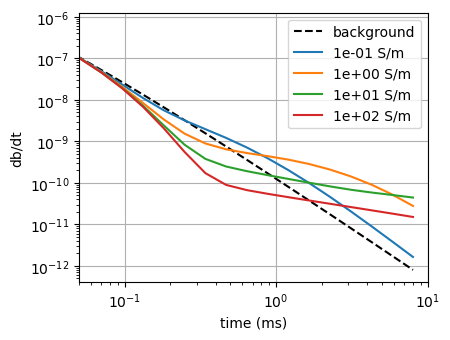
fig, ax = plt.subplots(1, 1, figsize=(4.5, 3.5))
highlight = None
for i, key in enumerate(dpred1d.keys()):
val = dpred1d[key]
if i == 0:
color = "--k"
label="background"
else:
color = f"C{i-1}"
label = f"{key.split('_')[-1]} S/m"
ax.loglog(rx_times*1e3, -val, color, label=label, alpha=1 if highlight == i or highlight is None else 0.2)
ax.set_xlim(5e-2, 10)
# ax.set_ylim(1e-14, 4e-10)
ax.legend()
ax.set_xlabel("time (ms)")
ax.set_ylabel("db/dt")
ax.grid()
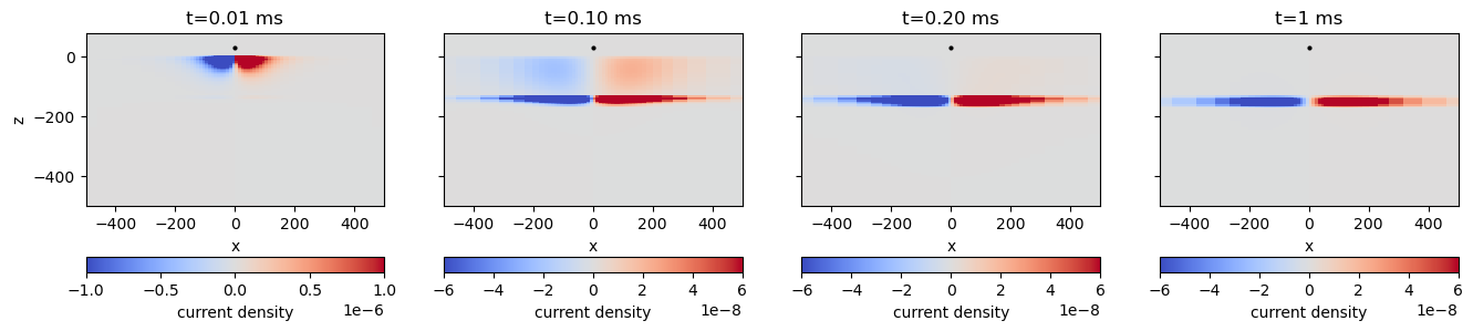
def plot_current_density(
    key, ti, ax=None, xlim = 500*np.r_[-1, 1], zlim=np.r_[-500, 80],
    colorbar=False, ylabels=True, vmax=None
):
    if ax is None:
        fig, ax = plt.subplots(1, 1, figsize=(4, 4))
    jplt = mesh.average_edge_y_to_cell * fields[key][:, "j", ti]

    if vmax is not None:
        pcolor_opts={"norm":Normalize(vmin=-vmax, vmax=vmax), "cmap":"coolwarm"}
    else:
        pcolor_opts = {"cmap":"coolwarm"}
    out = mesh.plot_image(
        jplt, ax=ax,
        mirror=True, mirror_data = -jplt,
        pcolor_opts=pcolor_opts
    )

    ax.plot(np.r_[0], tx_height, "ko", ms=2)
    ax.set_xlim(xlim)
    ax.set_ylim(zlim)
    ax.set_aspect(1)

    if colorbar is True:
        cb = plt.colorbar(out[0], ax=ax, orientation="horizontal")
        cb.set_label("current density")

    time_label = (sim.times[ti]-waveform.off_time)*1e3

    if ylabels is False:
        ax.set_ylabel("")
        ax.set_yticklabels("")

    if time_label > 0.99:
        ax.set_title(f"t={time_label:1.1f} ms")
    else:
        ax.set_title(f"t={time_label:1.2f} ms")

    return out
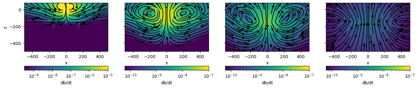
def plot_dbdt(
    key, ti, ax=None, xlim = 500*np.r_[-1, 1], zlim = np.r_[-500, 80],
    colorbar=False, ylabels=True, vmax=1e-6, vmin=1e-12
):
    dbdtplt = mesh.average_face_to_cell_vector * fields[key][:, "dbdt", ti]
    out = mesh.plot_image(
        dbdtplt, "CCv", view="vec", ax=ax,
        mirror=True,
        pcolor_opts={"norm":LogNorm(vmin=vmin, vmax=vmax)},
        range_x=xlim,
        range_y=zlim,
        stream_threshold=vmin
    )
    ax.plot(np.r_[0], tx_height, "ko", ms=2)
    ax.set_xlim(xlim)
    ax.set_ylim(zlim)
    ax.set_aspect(1)
    if ylabels is False:
        ax.set_ylabel("")
        ax.set_yticklabels("")
    if colorbar is True:
        cb = plt.colorbar(out[0], ax=ax, orientation="horizontal")
        cb.set_label("db/dt")
from matplotlib import animation, collectionstimes = np.where(sim.times > waveform.off_time-1e-6)[0]
timesarray([ 0, 1, 2, 3, 4, 5, 6, 7, 8, 9, 10, 11, 12,
13, 14, 15, 16, 17, 18, 19, 20, 21, 22, 23, 24, 25,
26, 27, 28, 29, 30, 31, 32, 33, 34, 35, 36, 37, 38,
39, 40, 41, 42, 43, 44, 45, 46, 47, 48, 49, 50, 51,
52, 53, 54, 55, 56, 57, 58, 59, 60, 61, 62, 63, 64,
65, 66, 67, 68, 69, 70, 71, 72, 73, 74, 75, 76, 77,
78, 79, 80, 81, 82, 83, 84, 85, 86, 87, 88, 89, 90,
91, 92, 93, 94, 95, 96, 97, 98, 99, 100])key = "sigma_1e-02"
times = np.where(sim.times*1e3 < 2)[0]
ims = []
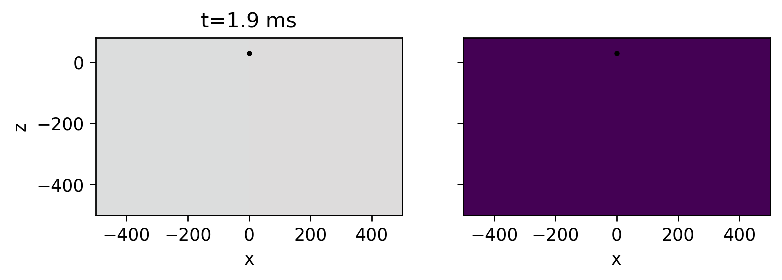
fig, ax = plt.subplots(1, 2, figsize=(7, 2), dpi=250)
def plotme(key, ti):
outj = plot_current_density(key, ti, ax=ax[0], vmax=2e-7)
outdbdt = plot_dbdt(key, ti, ax=ax[1], ylabels=False, vmin=6e-11, vmax=3e-7)
return np.hstack([outj, outdbdt])
out = plotme(key, 0)
def init():
[o.set_array(None) for o in out if isinstance(o, collections.QuadMesh)]
return out
def update(t):
for a in ax:
a.clear()
return plotme(key, t)
ani = animation.FuncAnimation(fig, update, times, init_func=init, blit=False)
ani.save(
f"./geotech-videos/currents_{key}.mp4", writer="ffmpeg", fps=3, bitrate=0,
metadata={"title":f"TDEM {key} currents", "artist":"Lindsey Heagy"}
)
# plot_times = [79, 80, 89, 119, 144]
# plot_times = [177, 178, 187, 248, 280]
plot_times = [1, 10, 20, 60]
(sim.times[plot_times] - waveform.off_time)*1e3
array([0.01, 0.1 , 0.2 , 1. ])key = "sigma_1e+00"
fig, ax = plt.subplots(1, len(plot_times), figsize=(4*len(plot_times), 4))
xlim = 500*np.r_[-1, 1]
zlim = np.r_[-500, 80]
# vmax = [1e-6, 3e-8, 2e-8, 3e-9]
vmax = [1e-6, 6e-8, 6e-8, 6e-8]
for i, ti in enumerate(plot_times):
out = plot_current_density(key, ti, ax=ax[i], vmax=vmax[i], colorbar=True)
time_label = (sim.times[ti]-waveform.off_time)*1e3
if time_label > 0.9:
ax[i].set_title(f"t={time_label:1.0f} ms")
else:
ax[i].set_title(f"t={time_label:1.2f} ms")
if i > 0:
ax[i].set_ylabel("")
ax[i].set_yticklabels("")
fig, ax = plt.subplots(1, len(plot_times), figsize=(4*len(plot_times), 4))
xlim = 500*np.r_[-1, 1]
zlim = np.r_[-500, 80]

vmax=[1e-5, 1e-7, 1e-7, 1e-7]
vmin=[3e-10, 6e-11, 6e-11, 6e-11]

for i, ti in enumerate(plot_times):
    dbdtplt = mesh.average_face_to_cell_vector * fields[key][:, "dbdt", ti]
    plot_dbdt(key, ti, ax=ax[i], vmax=vmax[i], vmin=vmin[i], colorbar=True)

    time_label = (sim.times[ti]-waveform.off_time)*1e3
    # if time_label > 0.9:
    #     ax[i].set_title(f"t={time_label:1.0f} ms")
    # else:
    #     ax[i].set_title(f"t={time_label:1.2f} ms")
    if i > 0:
        ax[i].set_ylabel("")
        ax[i].set_yticklabels("")
key = "sigma_1e-01"
data_invert = data.Data(survey, dobs=dpred[key], relative_error=0.02)
cs_invert = 5
inv_thicknesses = np.hstack([[cs_invert]*int(300/cs_invert), cs_invert * np.logspace(0, 1.5, 20)])mesh_invert = discretize.TensorMesh([(np.r_[inv_thicknesses, inv_thicknesses[-1]])], origin="0")mesh_invert
  TensorMesh: 81 cells

                      MESH EXTENT             CELL WIDTH      FACTOR
  dir    nC        min           max         min       max      max
  ---   ---  ---------------------------  ------------------  ------
   x     81          0.00      1,384.28      5.00    158.11    1.20
target_zarray([-165., -135.])# waveform=tdem.sources.VTEMWaveform()
rx_z = tdem.receivers.PointMagneticFluxTimeDerivative(
np.r_[0, 0, tx_height], times=rx_times, orientation="z"
)
src = tdem.sources.CircularLoop(
location=np.r_[0, 0, tx_height], radius=tx_radius, receiver_list=[rx_z], #waveform=waveform
)
survey_invert = tdem.Survey([src])
sim1d = tdem.Simulation1DLayered(
survey=survey, thicknesses=inv_thicknesses, sigmaMap=maps.ExpMap(mesh_invert)
)np.diff(target_z)array([30.])#
m_true = np.log(np.r_[1./rho_back, 0.1, 1./rho_back])
sim1d_true = tdem.Simulation1DLayered(
survey=tdem.Survey([src]), thicknesses=np.r_[-target_z.max(), np.diff(target_z)], sigmaMap=maps.ExpMap(nP=3)
)
dobs = sim1d_true.dpred(m_true)
data_invert = data.Data(survey, dobs=dobs, relative_error=0.05)plt.loglog(rx_times, -dobs)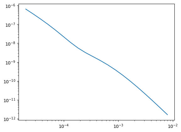
def setup_inversion(norms=[0, 0]):
    dmis = data_misfit.L2DataMisfit(simulation=sim1d, data=data_invert)
    reg = regularization.Sparse(
        mesh_invert, alpha_s=0.1, alpha_x=1.0,
        reference_model=np.log(1./rho_back),
        norms=norms
    )

    opt = optimization.InexactGaussNewton(maxIter=30, tolCG=1e-3)
    inv_prob = inverse_problem.BaseInvProblem(dmis, reg, opt)

    # Defining a starting value for the trade-off parameter (beta) between the data
    # misfit and the regularization.
    starting_beta = directives.BetaEstimate_ByEig(beta0_ratio=1e1)

    # Update the preconditionner
    update_Jacobi = directives.UpdatePreconditioner()

    # Options for outputting recovered models and predicted data for each beta.
    save_iteration = directives.SaveOutputEveryIteration(save_txt=False)

    # Directives for the IRLS
    update_IRLS = directives.Update_IRLS(
        max_irls_iterations=30, minGNiter=1, coolEpsFact=1.5, update_beta=True
    )

    # Updating the preconditionner if it is model dependent.
    update_jacobi = directives.UpdatePreconditioner()

    # Add sensitivity weights
    sensitivity_weights = directives.UpdateSensitivityWeights()

    # The directives are defined as a list.
    directives_list = [
        sensitivity_weights,
        starting_beta,
        save_iteration,
        update_IRLS,
        update_jacobi,
    ]

    # Here we combine the inverse problem and the set of directives
    inv = inversion.BaseInversion(inv_prob, directives_list)

    return inv
invl1 = setup_inversion([1, 1])
# Run the inversion
starting_model = np.log(1./rho_back)*np.ones(mesh_invert.n_cells)
recovered_model_l1 = invl1.run(starting_model)
                        SimPEG.InvProblem is setting bfgsH0 to the inverse of the eval2Deriv.
                        ***Done using same Solver, and solver_opts as the Simulation1DLayered problem***

model has any nan: 0
============================ Inexact Gauss Newton ============================
  #     beta     phi_d     phi_m       f      |proj(x-g)-x|  LS    Comment
-----------------------------------------------------------------------------
x0 has any nan: 0
   0  4.09e+03  6.52e+02  0.00e+00  6.52e+02    1.37e+02      0
   1  2.05e+03  5.81e+02  7.35e-03  5.96e+02    8.72e+01      0
   2  1.02e+03  4.60e+02  4.77e-02  5.09e+02    6.67e+01      0   Skip BFGS
   3  5.12e+02  3.35e+02  1.55e-01  4.14e+02    6.27e+01      0   Skip BFGS
   4  2.56e+02  2.00e+02  4.07e-01  3.04e+02    5.34e+01      0   Skip BFGS
   5  1.28e+02  1.01e+02  8.04e-01  2.04e+02    4.04e+01      0   Skip BFGS
   6  6.40e+01  4.70e+01  1.27e+00  1.28e+02    2.72e+01      0   Skip BFGS
   7  3.20e+01  2.09e+01  1.74e+00  7.65e+01    1.60e+01      0   Skip BFGS
Reached starting chifact with l2-norm regularization: Start IRLS steps...
irls_threshold 1.464513579084576
   8  1.60e+01  9.30e+00  2.46e+00  4.86e+01    7.48e+00      0   Skip BFGS
   9  3.83e+01  3.58e+00  3.29e+00  1.30e+02    3.64e+01      0
  10  3.16e+01  1.11e+01  2.81e+00  9.97e+01    4.14e+00      0
  11  5.01e+01  8.52e+00  3.18e+00  1.68e+02    2.53e+01      0
  12  3.44e+01  1.60e+01  2.99e+00  1.19e+02    1.50e+01      0
  13  5.39e+01  8.86e+00  3.52e+00  1.98e+02    2.96e+01      0
  14  3.52e+01  1.80e+01  3.23e+00  1.31e+02    2.12e+01      0
  15  5.54e+01  8.72e+00  3.76e+00  2.17e+02    3.22e+01      0
  16  3.54e+01  1.89e+01  3.37e+00  1.38e+02    2.48e+01      0
  17  5.62e+01  8.52e+00  3.89e+00  2.27e+02    3.35e+01      0
  18  3.57e+01  1.91e+01  3.43e+00  1.42e+02    2.64e+01      0
  19  5.71e+01  8.37e+00  3.92e+00  2.32e+02    3.42e+01      0
  20  3.63e+01  1.92e+01  3.44e+00  1.44e+02    2.69e+01      0
  21  5.81e+01  8.34e+00  3.91e+00  2.35e+02    3.47e+01      0
  22  3.68e+01  1.93e+01  3.43e+00  1.46e+02    2.71e+01      0
  23  5.89e+01  8.36e+00  3.88e+00  2.37e+02    3.49e+01      0
  24  3.73e+01  1.94e+01  3.41e+00  1.46e+02    2.73e+01      0
  25  5.95e+01  8.39e+00  3.86e+00  2.38e+02    3.48e+01      0
  26  3.77e+01  1.94e+01  3.38e+00  1.47e+02    2.73e+01      0
  27  6.00e+01  8.43e+00  3.83e+00  2.38e+02    3.47e+01      0
  28  3.80e+01  1.94e+01  3.36e+00  1.47e+02    2.73e+01      0
  29  6.04e+01  8.46e+00  3.79e+00  2.38e+02    3.43e+01      0
  30  3.82e+01  1.94e+01  3.34e+00  1.47e+02    2.72e+01      0
------------------------- STOP! -------------------------
0 : |fc-fOld| = 9.0641e+01 <= tolF*(1+|f0|) = 6.5316e+01
1 : |xc-x_last| = 1.7538e-01 <= tolX*(1+|x0|) = 4.2447e+00
0 : |proj(x-g)-x|    = 2.7207e+01 <= tolG          = 1.0000e-01
0 : |proj(x-g)-x|    = 2.7207e+01 <= 1e3*eps       = 1.0000e-02
1 : maxIter   =      30    <= iter          =     30
------------------------- DONE! -------------------------
invl0 = setup_inversion([0, 0])
recovered_model_l0 = invl0.run(starting_model)
                        SimPEG.InvProblem is setting bfgsH0 to the inverse of the eval2Deriv.
                        ***Done using same Solver, and solver_opts as the Simulation1DLayered problem***

model has any nan: 0
============================ Inexact Gauss Newton ============================
  #     beta     phi_d     phi_m       f      |proj(x-g)-x|  LS    Comment
-----------------------------------------------------------------------------
x0 has any nan: 0
   0  4.77e+03  6.52e+02  0.00e+00  6.52e+02    1.37e+02      0
   1  2.39e+03  5.92e+02  5.31e-03  6.05e+02    8.84e+01      0
   2  1.19e+03  4.83e+02  3.60e-02  5.26e+02    6.72e+01      0   Skip BFGS
   3  5.97e+02  3.65e+02  1.21e-01  4.37e+02    6.39e+01      0   Skip BFGS
   4  2.98e+02  2.28e+02  3.36e-01  3.28e+02    5.59e+01      0   Skip BFGS
   5  1.49e+02  1.19e+02  7.08e-01  2.24e+02    4.34e+01      0   Skip BFGS
   6  7.46e+01  5.60e+01  1.16e+00  1.43e+02    3.00e+01      0   Skip BFGS
   7  3.73e+01  2.50e+01  1.64e+00  8.60e+01    1.82e+01      0   Skip BFGS
   8  1.86e+01  1.11e+01  2.11e+00  5.04e+01    9.56e+00      0   Skip BFGS
Reached starting chifact with l2-norm regularization: Start IRLS steps...
irls_threshold 1.5640160800030474
   9  9.32e+00  5.04e+00  2.96e+00  3.26e+01    4.84e+00      0   Skip BFGS
  10  3.24e+01  2.02e+00  3.12e+00  1.03e+02    4.32e+01      0
  11  8.44e+01  3.12e+00  2.27e+00  1.94e+02    5.32e+01      0
  12  1.37e+02  8.05e+00  1.66e+00  2.35e+02    4.90e+01      0
  13  1.06e+02  1.26e+01  1.20e+00  1.39e+02    3.17e+01      0
  14  2.32e+02  4.19e+00  9.36e-01  2.21e+02    5.96e+01      0
  15  2.32e+02  1.05e+01  5.88e-01  1.47e+02    3.45e+01      0
  16  4.66e+02  4.94e+00  4.07e-01  1.95e+02    5.50e+01      0
  17  7.41e+02  8.46e+00  2.54e-01  1.97e+02    6.13e+01      0
  18  7.41e+02  9.55e+00  1.66e-01  1.32e+02    3.80e+01      0
  19  1.58e+03  4.42e+00  1.16e-01  1.87e+02    4.86e+01      0
  20  2.53e+03  8.29e+00  7.33e-02  1.94e+02    5.41e+01      0
  21  2.53e+03  9.18e+00  4.83e-02  1.32e+02    7.78e+01      0   Skip BFGS
  22  4.78e+03  5.64e+00  3.32e-02  1.65e+02    6.76e+01      0
  23  8.76e+03  6.02e+00  2.20e-02  1.99e+02    1.14e+02      0
  24  1.51e+04  6.92e+00  1.45e-02  2.26e+02    2.36e+02      0
  25  2.46e+04  7.91e+00  9.58e-03  2.44e+02    2.51e+02      0
  26  3.85e+04  8.83e+00  6.33e-03  2.53e+02    3.73e+02      0
  27  3.85e+04  9.75e+00  4.19e-03  1.71e+02    3.93e+02      0
  28  6.37e+04  7.66e+00  2.85e-03  1.89e+02    8.54e+01      0
  29  1.06e+05  7.56e+00  1.90e-03  2.08e+02    1.57e+03      0   Skip BFGS
  30  1.71e+05  8.08e+00  1.26e-03  2.24e+02    1.48e+03      0
------------------------- STOP! -------------------------
1 : |fc-fOld| = 1.5150e+01 <= tolF*(1+|f0|) = 6.5316e+01
1 : |xc-x_last| = 2.2667e-02 <= tolX*(1+|x0|) = 4.2447e+00
0 : |proj(x-g)-x|    = 1.4806e+03 <= tolG          = 1.0000e-01
0 : |proj(x-g)-x|    = 1.4806e+03 <= 1e3*eps       = 1.0000e-02
1 : maxIter   =      30    <= iter          =     30
------------------------- DONE! -------------------------
invl0.fig, ax = plt.subplots(1, 1, figsize=(3, 5))
plot_1d_layer_model(sim1d_true.thicknesses, np.exp(m_true), ax=ax, color="k", label="True")
plot_1d_layer_model(mesh_invert.h[0], np.exp(invl0.invProb.l2model), ax=ax, label="L2")
plot_1d_layer_model(mesh_invert.h[0], np.exp(recovered_model_l1), ax=ax, label="L1")
plot_1d_layer_model(mesh_invert.h[0], np.exp(recovered_model_l0), ax=ax, label="L0")
ax.set_ylim([450, 0])
ax.set_xlim([6e-3, 2e-1])
ax.grid("both", alpha=0.7)
ax.legend()
ax.set_xlabel("conductivity (S/m)")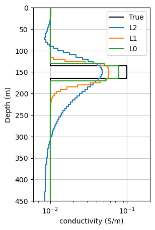
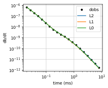
fig, ax = plt.subplots(1, 1, figsize=(3.5, 3))

ax.loglog(rx_times*1e3, -dobs, "ko", label="dobs", ms=4)
ax.loglog(rx_times*1e3, -sim1d.dpred(invl0.invProb.l2model), label="L2")
ax.loglog(rx_times*1e3, -sim1d.dpred(recovered_model_l1), label="L1")
ax.loglog(rx_times*1e3, -sim1d.dpred(recovered_model_l0), label="L0")

ax.legend()
ax.grid("both", alpha=0.7)
ax.set_xlabel("time (ms)")
ax.set_ylabel("db/dt")